SCR Calculator User Manual

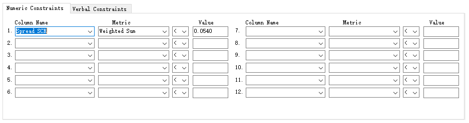
Step 4: Add Numeric Constraint(s)

Start by selecting "Spread SCR" in the "Column Name" field of the first numeric constraint row. The "Metric" field will automatically populate with "Weighted Sum", the calculation method for this metric based on the calculator's interpretation or any prior definition. The "Value" field will also auto-fill with 0.0540, which represents the current allocation's Spread SCR. Leave this value unchanged to set it as a cap for the next optimisation step.

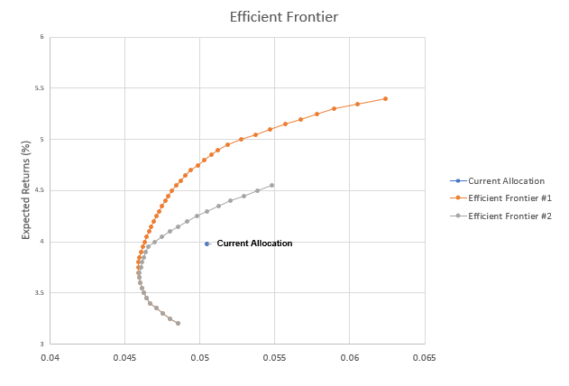
Click the "Run EF Calibration" button again. This generates EF #2 (yellow), which is lower than EF #1 but still above the current allocation:

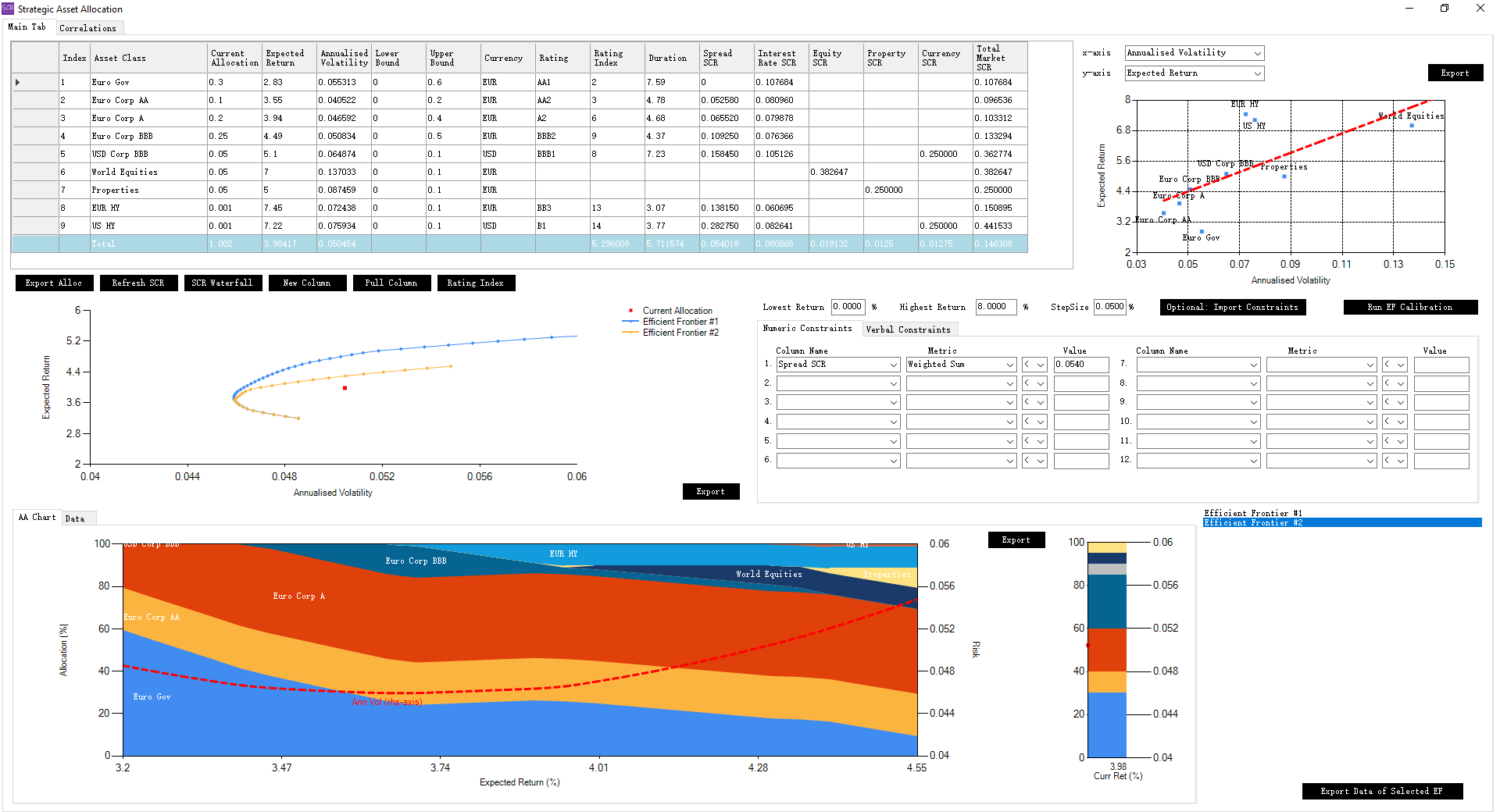
Selecting any efficient frontier updates the entire form to reflect its original settings. This allows you to replicate and compare different frontiers with precision.

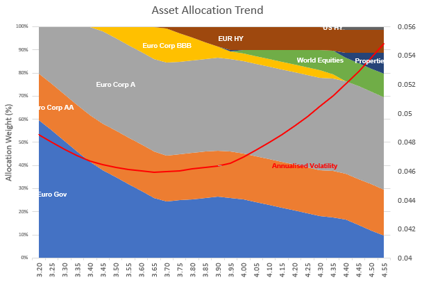
The stacked area "AA Chart" visualises allocation trends across different expected return levels (X-axis).

Both the Efficient Frontier chart and the AA Chart can be exported as PowerPoint slides. Below are examples of exported slides:

• "Weighted Average": Values are multiplied by their weights, summed, and then divided by the total weight.
• "Weighted Sum": Values are multiplied by their weights and summed, without dividing by the total weight.
• These metrics yield identical results when the total weight is 100%, but differ when it is not.

When applying a constraint to duration, if fixed income asset allocations are already heavily bounded, you can use "Weighted Average". Otherwise, use "Weighted Sum" to ensure the duration constraint remains valid even if fixed income asset weights shift.