SCR Calculator User Manual

Step 3: Generate an Efficient Frontier

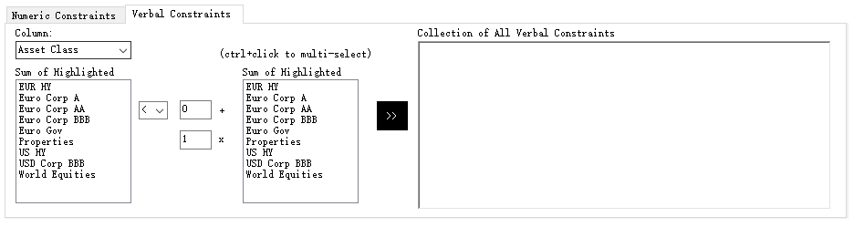
After importing your data, you’ll notice a Constraint Setting Panel has appeared on the right-hand side of the form. It includes two tabs: "Numeric Constraints" and "Verbal Constraints", as shown below:

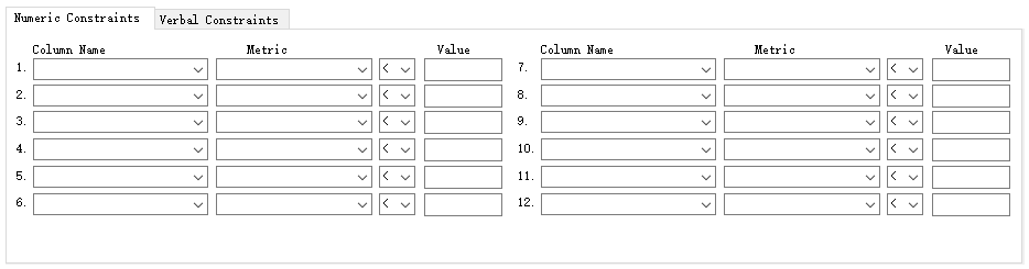
For now, ignore these tabs and click the "Run EF Calibration" button on the right side of the form. This will generate an efficient frontier, as shown below:

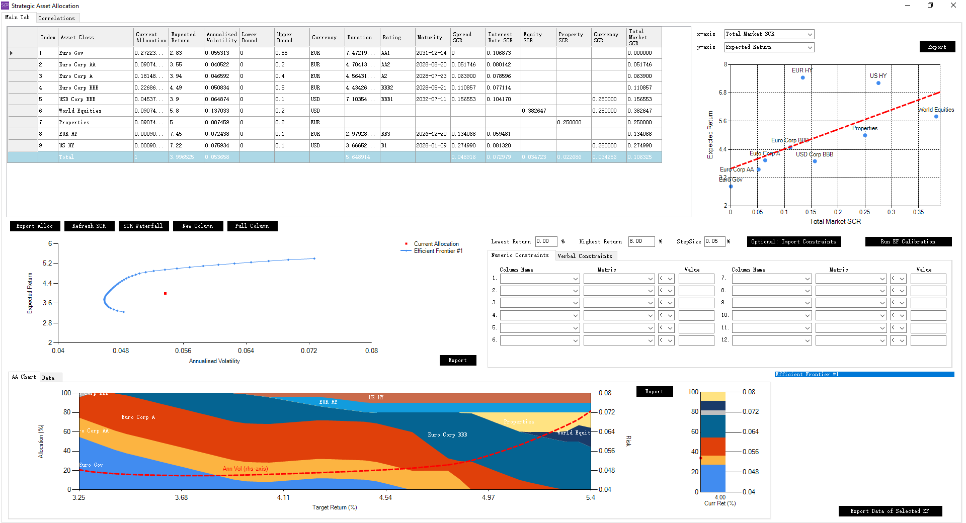
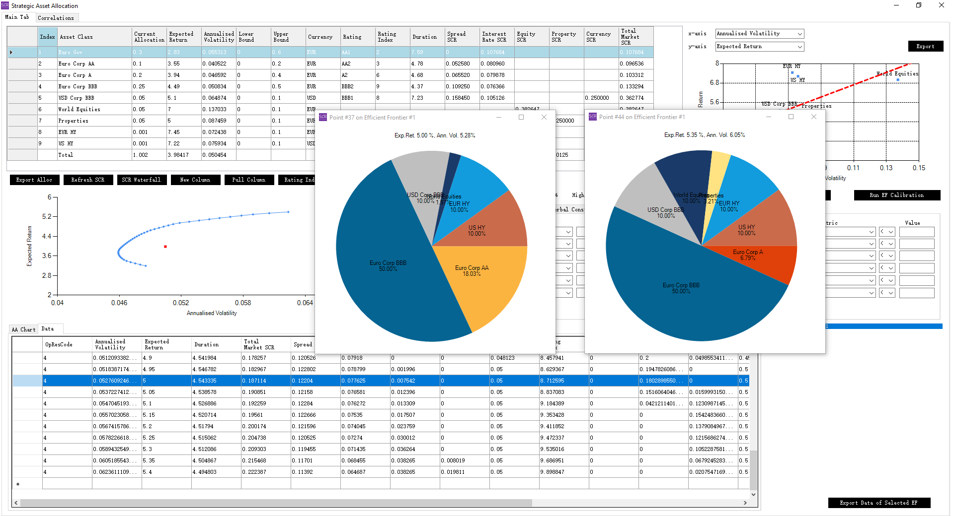
Clicking on any point on the efficient frontier will display pie charts with the corresponding risk, return, and allocation breakdowns:

To evaluate the impact of adding high-yield asset classes, adjust the Upper Bounds for EUR HY and US HY to zero (individually and together), and re-run the optimisation each time. This will produce lower efficient frontiers (e.g., #2, #3, #4) as shown below:

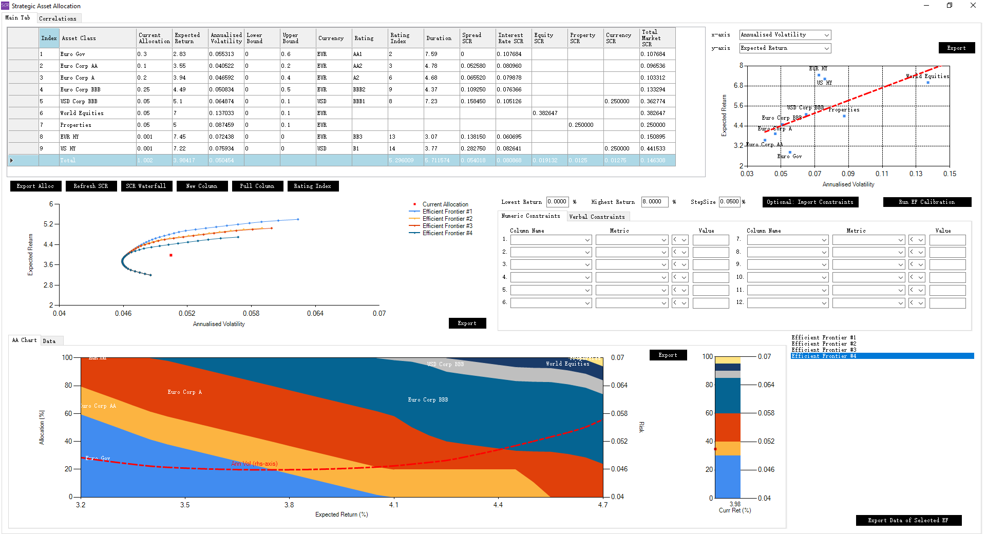
The expanded efficient frontier (#1) demonstrates the value of new asset classes. Comparing frontiers #2 and #3 suggests that EUR HY and US HY provide similar risk-return improvements.

The tool keeps a history of efficient frontiers in a list on the bottom right. Clicking on a frontier will refresh the form to reflect that specific frontier. You can delete frontiers #2, #3, and #4 to revert the form to frontier #1.

With frontier #1, you can perform further investigations:

• Hover over any point on the frontier to view its exact risk/return values.
• Switch to the "Data" tab (next to "AA Chart") to view a detailed table of metrics: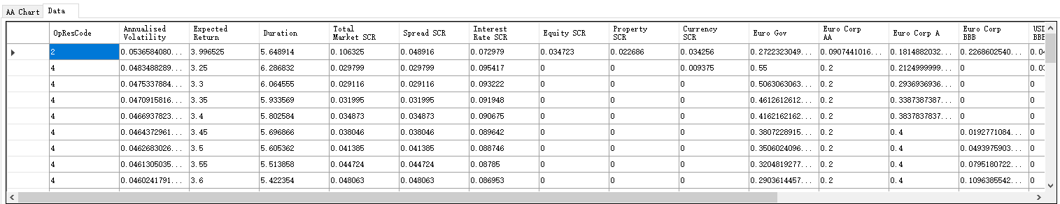
  
  • Each row represents a point on the efficient frontier. Clicking a point highlights the corresponding row and updates the pie chart.
  • The "OpResCode" column indicates the optimisation status:
    • "1": Minimal relative function improvement (EpsF).
    • "2": Minimal relative step size (EpsX).
    • "4": Gradient norm below threshold (EpsG).
    • "5": Maximum iterations reached (MaxIts).
    • "7": Constraints too stringent, best point found so far.
    • "8": Terminated by user with the best current point recorded.
  • Metrics such as volatility, return, duration, and other user-defined numeric columns are automatically calculated and available for review or setting constraints.

On the right, a list of efficient frontiers includes an "Export Data of Selected EF" button, which exports a detailed spreadsheet with multiple tabs:

• "ALLOC": Allocation table copy.
• "TRS": Total Return Series data.
• "SETTINGS": Expected returns, step sizes, and related settings.
• "NCON": Numeric constraints (empty if none).
• "VCON": Verbal constraints (empty if none).
• "CORR": Correlation matrix.
• "EF": Efficient frontier data.

This spreadsheet serves as a complete definition of the efficient frontier and can be reused as an input sheet to regenerate it. Use the "Optional: Import Constraints" button to reapply saved constraints if needed.